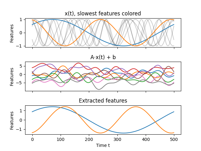
Randomly Mapped Cosines

An example plot of sksfa.SFA applied to randomly mixed and shifted cosines. SFA is able to recover the slowest of the underlying signals perfectly, except for sign and offset.

import numpy as np
from sksfa import SFA
import matplotlib.pyplot as plt


n_samples = 500
dim = 8
n_slow_features = 2

# Generate different randomly shifted time-scales
t = np.linspace(0, 2*np.pi, n_samples).reshape(n_samples, 1)
t = t * np.arange(1, dim+1)
t += np.random.uniform(0, 2*np.pi, (1, dim))

# Generate latent cosine signals
x = np.cos(t)

# Compute random affine mapping of cosines (observed)
A = np.random.normal(0, 1, (dim, dim))
b = np.random.normal(0, 2, (1, dim))
data = np.dot(x, A) + b

# Extract slow features from observed data
sfa = SFA(n_slow_features)
slow_features = sfa.fit_transform(data)

# Plot cosines, mapped data, and extracted features
fig, ax = plt.subplots(3, 1, sharex=True)
fig.subplots_adjust(hspace=0.5)
for d in reversed(range(n_slow_features, dim)):
    ax[0].plot(x[:, d], color=(0.2, 0.2, 0.2, 0.25))
for d in range(n_slow_features):
    ax[0].plot(x[:, d])
ax[1].plot(data)
ax[2].plot(slow_features)
ax[0].set_title("x(t), slowest features colored")
ax[1].set_title("A⋅x(t) + b")
ax[2].set_title("Extracted features")
ax[2].set_xlabel("Time t")
for idx in range(3):
    ax[idx].set_ylabel("Features")
plt.show()